How to Combine Uncorrelated Trading Strategies
Why several weak but uncorrelated trading strategies can beat one strong one, the portfolio Sharpe formula, and when adding a sleeve dilutes the book.
Part 18 of 20 · How to Algo · Previous: Position sizing · Next: Backtest vs live
The most reliable way we know to improve a trading book is not a better signal. It is another signal that is mediocre on its own and uncorrelated with what you already run. Edges that survive honest testing tend to be modest: Sharpe ratios well under 1 for a single strategy are normal. Combined correctly, several of them can do what none can alone.
The catch is the word “uncorrelated”. It is easy to believe you hold five strategies when you hold one strategy five times.
The formula
For N strategies with the same Sharpe S, the same risk weight and the same pairwise correlation ρ:
portfolio Sharpe = S × √N / √(1 + (N − 1) × ρ)
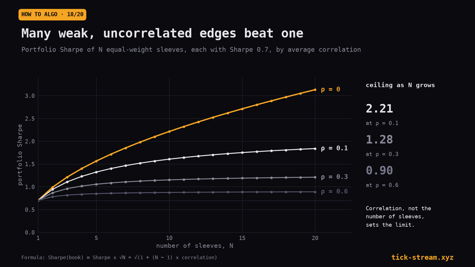
With ρ = 0 this grows with √N. With ρ > 0 it flattens and approaches a ceiling of S / √ρ no matter how many strategies you add.
For strategies with a Sharpe of 0.6 each:
| Strategies | ρ = 0 | ρ = 0.1 | ρ = 0.2 | ρ = 0.3 | ρ = 0.5 |
|---|---|---|---|---|---|
| 1 | 0.60 | 0.60 | 0.60 | 0.60 | 0.60 |
| 3 | 1.04 | 0.95 | 0.88 | 0.82 | 0.73 |
| 5 | 1.34 | 1.13 | 1.00 | 0.90 | 0.77 |
| 10 | 1.90 | 1.38 | 1.13 | 0.99 | 0.81 |
| 20 | 2.68 | 1.58 | 1.22 | 1.04 | 0.83 |
Two lessons are in this table. First, five independent strategies at 0.6 beat one strategy at 1.2, and are far easier to find. Second, correlation is expensive: at 0.3, twenty strategies barely beat five independent ones. The chart above draws the same curves for sleeves of Sharpe 0.7: the ceiling is 2.21 at a correlation of 0.1, 1.28 at 0.3 and 0.90 at 0.6.
When adding a strategy helps
The general rule, for adding strategy B to a portfolio A at the best weight: B improves the portfolio if its Sharpe is greater than its correlation with A times A’s Sharpe.
- A portfolio with Sharpe 1.0 and a candidate with correlation 0.3 needs the candidate’s Sharpe above 0.3.
- With correlation 0.05, a candidate with Sharpe 0.1 already helps, at the right weight.
- With correlation 0.7, the candidate needs a Sharpe above 0.7, close to the portfolio itself.
This is why a weak, uncorrelated strategy is often worth more than a strong, correlated one. It is also why “at the best weight” carries so much of the meaning.
Three cases from our own book
A duplicate disguised as diversification. RSI-2 dip buying works on both ES and NQ. Running both looks like two markets. Their daily P&L correlated 0.51, and 65.4% of entries fell on the same days. Stacking them lowered return over drawdown from 9.49 to 8.44. It is the same trade on two highly correlated indices, taken twice. The ES RSI-2 test recommends one or the other.
The same check closed another idea. A one-day reversal rule on NQ was real and tradable on its own, and correlated +0.69 with a sleeve we already ran. We already owned that factor; adding it would have doubled the position, not diversified it.
An uncorrelated sleeve that still diluted the book. Gold’s overnight drift was a robust attribution in our data: the metal gained during Asian hours and gave part of it back in New York. As a strategy it had a Sharpe of about 0.44 and a correlation of only 0.06 with the stronger gold sleeve we combined it with. By the rule above it should have helped. At every contract weight we tried, it diluted the combination, and more so the larger the weight. The reason was risk weight: held overnight on full contracts, the drift sleeve carried more dollar volatility than the sleeve it was meant to diversify, so its low Sharpe dominated the mix. Combined by risk instead of by contracts, the arithmetic changes; combined by contracts, it was a mistake.
A portfolio inherits the bugs of its parts. In June 2026 our backtested book of seven sleeves showed a Sharpe of about 2.3, far above any single sleeve, precisely because of the diversification above. The value was real only to the extent each sleeve’s backtest was real. When we rebuilt the live paper record of June and July by replaying archived ticks through the production code, the book went from +$5,145 to −$65,725, mostly through fill and data errors in individual sleeves (Part 19). Diversification multiplies honest edges and dishonest ones alike.
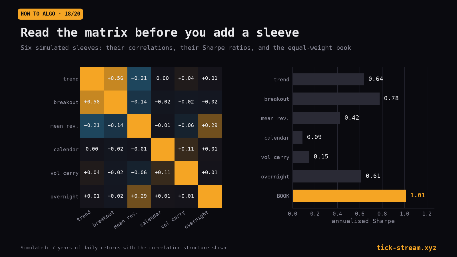
In the simulated six-sleeve example above, no sleeve reaches 0.8 on its own and the equal-weight book reaches 1.01. The matrix also shows which pair to question first: trend and breakout at +0.56 are closer to one position than two.
Measure correlation the right way
- Use daily P&L, including zero days, not trade-level returns. Strategies that trade on different days can still share risk through the days they do trade.
- Check entry overlap. The share of days on which both strategies enter is a direct measure of duplication.
- Look at the bad days. Correlation on the worst 5% of days for the portfolio, or during its drawdowns, is often higher than the average. Strategies that share a hidden exposure, such as being long the index or short volatility, lose together exactly when it hurts.
- Use enough history. Correlation estimates from one year are noisy; a correlation of 0.1 and 0.3 can be hard to tell apart on short samples.
Weight by risk
The simplest robust weighting is equal risk: size each strategy so that it contributes a similar expected dollar volatility (Part 17 covers the sizing). It avoids letting the most volatile strategy dominate, which is exactly what went wrong with the gold drift sleeve.
Optimised weights (maximising the in-sample portfolio Sharpe) are tempting and fragile. They load up on whichever strategy had the best backtest, which is usually the one with the largest selection bias. Equal risk, perhaps tilted modestly toward strategies with longer, cleaner track records, is harder to fool.
Diversify mechanisms, not parameters
Five variants of the same idea with different parameters are not five strategies. Neither are the same rule on ES, NQ and RTY. Diversification comes from different mechanisms: mean reversion over days, trend over months, volatility-regime timing, calendar-driven flows. A breakout sleeve we run correlated about −0.05 with our trend sleeve, because the two respond to different things, and our options-positioning sleeve correlated −0.04 with an RSI-2-style dip-buying sleeve. That is the kind of pair that makes the formula work.
Every sleeve must pass on its own first
The formula rewards adding strategies, which creates a temptation: lower the bar for each new sleeve because “the portfolio will diversify it”. That reverses the logic. Diversification reduces the noise of honest edges; it does nothing for a sleeve whose backtest is an artefact, and it makes the artefact harder to see, because its losses are diluted by the others. Each sleeve should pass costs, significance, a placebo, a holdout and a live reconciliation on its own before it earns a place in the book.
Correlations also need watching after launch. Recompute them on live P&L at regular intervals and compare with the backtest’s values. A pair that drifts from near zero toward 0.5 is turning into one position, and the book’s risk has grown without any change in sizing.
Checklist
- Compute daily P&L correlations between every pair of strategies, including zero days.
- Measure the overlap of entry days.
- Check correlations on the portfolio’s worst days.
- Before adding a strategy, check that its Sharpe exceeds its correlation with the book times the book’s Sharpe.
- Weight strategies by risk, not by contracts.
- Prefer equal-risk weights over optimised ones.
- Diversify by mechanism, not by parameter or instrument.
- Remember that a portfolio backtest is only as honest as its least honest sleeve.
A portfolio of honest backtests still has to survive contact with live trading, and the differences are where the remaining bugs live. Part 19: Backtest vs live trading, paper trading and reconciliation.
Frequently asked questions
Does combining uncorrelated strategies improve the Sharpe ratio?
Yes, if they are really uncorrelated. For N strategies with the same Sharpe S, equal risk and the same pairwise correlation ρ, the portfolio Sharpe is S × √N / √(1 + (N − 1)ρ). Five independent strategies at Sharpe 0.6 combine to about 1.34; with correlation 0.5, the same five combine to only about 0.77.
When does adding a strategy improve a portfolio?
When its Sharpe ratio is higher than its correlation with the portfolio times the portfolio's Sharpe, and it is added at a sensible risk weight. A weak but uncorrelated strategy clears that bar easily; a strong strategy highly correlated with what you already hold may not. The weight matters as much as the inclusion.
How many trading strategies should you run at once?
Correlation decides more than the count. With pairwise correlation ρ the portfolio Sharpe approaches a ceiling of S / √ρ however many strategies you add: at Sharpe 0.6 and ρ = 0.3, twenty strategies reach about 1.04 against 0.90 for five. A new, independent mechanism is worth more than another variant of one you already run.
Can adding an uncorrelated strategy make a portfolio worse?
Yes, if it is sized wrongly. A gold overnight sleeve we tested had a correlation of 0.06 with a stronger sleeve and still diluted the combination at every contract weight we tried, because at those weights its dollar volatility dominated the mix. Combine strategies by risk, not by contract count.
How do I know two strategies are really different?
Measure the correlation of their daily P&L and the overlap of their trading days. Our RSI-2 rule on ES and NQ looked like two markets, but daily P&L correlated 0.51 and 65.4% of entries fell on the same days; stacking them lowered return over drawdown from 9.49 to 8.44. That is one trade taken twice.