Twenty-Two Calendar Effects on the S&P, and Not One Survives Being Counted
We measured 22 calendar cells across 3,223 ES sessions from 2014 to 2026. Monday looks like the winner at $223.19 a session and t = 2.75, November at $300.59 and t = 2.68. Then we ran the same 22 cell shapes against 1,000 shuffles of the same returns: the best cell on shuffled data averages |t| = 2.72, and 41.1% of shuffled runs beat our real best. The famous turn-of-month effect pays $77.20 against $94.37 for ordinary days, which is the wrong way round.
We measured 22 calendar cells on 12.5 years of S&P futures: expiry weeks, weekdays, turn of month, every month of the year. Several look tradeable. Monday pays $223.19 a session, November $300.59. Then we ran the same 22 cell shapes against 1,000 shuffles of the same daily returns. The best cell on shuffled data averaged |t| = 2.72, and 41.1% of shuffles beat our real best outright.
That is the whole article. Not one of the 22 survives being counted as one of 22. The two effects our internal NQ work treated most kindly, post-expiry weeks and a Monday tilt, are the ones the longer S&P archive declines to confirm.
The prior we brought in
A calendar effect should only exist where somebody has to trade on a date whether they want to or not. Index funds rebalance on a schedule published in advance. Options dealers re-hedge after monthly expiry because the gamma they were hedging stops existing. Pension flows arrive at month end because that is when contributions clear.
That is forced flow, and it is the only mechanism on this list that survives being asked why. Everything else — the Monday mood, the September curse, the Santa rally — is folklore with a chart attached. We tested the folklore anyway, because the folklore is what gets sold.
The rule
- ES daily bars built from our own tick archive, New York time, 3 January 2014 to 10 September 2026, 3,223 sessions.
- Each session’s P&L is close to close on one contract: the previous close to this open, plus this open to this close. No stop, no filter, no selection.
- Expiry week is the Monday-to-Friday block ending on the third Friday, 745 sessions. Week after expiry is the Monday, Tuesday and Wednesday that follow it, 448 sessions. Everything else is “other”.
- Turn of month is calendar days 26 and later plus days 1 to 3.
- The baseline is every session in the window, which is what any cell has to beat.
- One contract throughout. Every cell is a hold, not a trade, so no cost is charged inside a cell; the standing series convention for a real round trip is $4.50 commission plus two ticks, which on ES is $29.50.
The baseline first
The single most common error in calendar research is comparing a cell to zero. The S&P drifts up. Any long-only bucket of S&P sessions is expected to be positive, so positive is not a finding.
| Every session, 2014–2026 | |
|---|---|
| Sessions | 3,223 |
| Average per session | $89.65 |
| Total, one contract | $288,950 |
| Sessions up | 54.3% |
| t | 2.49 (p = 0.0129) |
$89.65 a session is the line. A cell that pays $95 is not an effect, it is the market.
The cells that look real
Monday is the standout. It pays 2.5 times the baseline and is up 58.6% of the time, on 642 observations, which is not a small sample.
| Weekday | Sessions | Average | Up | t | p |
|---|---|---|---|---|---|
| Monday | 642 | $223.19 | 58.6% | 2.75 | 0.0061 |
| Tuesday | 657 | $55.10 | 51.4% | 0.77 | 0.4401 |
| Wednesday | 650 | $154.37 | 56.2% | 1.87 | 0.0623 |
| Thursday | 647 | −$40.34 | 52.2% | −0.49 | 0.6258 |
| Friday | 625 | $54.30 | 53.1% | 0.64 | 0.5229 |
Thursday is the only negative weekday at −$40.34. Note that it comes with a 52.2% up rate, which is the shape you get when a few large down sessions land on one weekday rather than when a weekday is genuinely bearish.
The month table is where a reader is most likely to talk themselves into something, so here it is in full rather than as two selected rows.
| Month | Sessions | Average | Up | t | p |
|---|---|---|---|---|---|
| Jan | 266 | $66.40 | 54.1% | 0.65 | 0.5175 |
| Feb | 259 | −$23.84 | 55.2% | −0.20 | 0.8403 |
| Mar | 280 | −$45.31 | 49.3% | −0.25 | 0.8003 |
| Apr | 267 | $132.40 | 56.2% | 0.74 | 0.4584 |
| May | 283 | $190.77 | 55.8% | 1.73 | 0.0852 |
| Jun | 277 | $145.89 | 56.7% | 1.17 | 0.2430 |
| Jul | 286 | $201.92 | 57.7% | 2.33 | 0.0206 |
| Aug | 283 | $78.45 | 52.3% | 0.73 | 0.4650 |
| Sep | 265 | −$108.49 | 49.4% | −1.01 | 0.3138 |
| Oct | 266 | $97.79 | 52.3% | 0.87 | 0.3874 |
| Nov | 255 | $300.59 | 61.6% | 2.68 | 0.0079 |
| Dec | 236 | $27.70 | 51.3% | 0.23 | 0.8168 |
November and July are the two that clear p = 0.05. Twelve months were measured to find them.
Post-expiry does not replicate
Expiry is the one cell on this list with a named mechanism behind it. Dealers who were hedging a book of expiring options stop hedging it, and the flow that suppressed movement goes away. Our own NQ run found the week after expiry to be a modest survivor. That run is internal and unpublished, so this is the first time we have put the test on the record.
| Around monthly expiry | Sessions | Average | Up | t | p |
|---|---|---|---|---|---|
| Expiry week | 745 | $52.95 | 53.2% | 0.72 | 0.4720 |
| Week after expiry | 448 | $134.93 | 55.8% | 1.56 | 0.1184 |
| Other weeks | 2,030 | $93.13 | 54.4% | 1.99 | 0.0463 |
The ordering is what the theory predicts. Expiry week is the weakest at $52.95, the week after is the strongest at $134.93. But t = 1.56 does not clear significance, and 448 sessions is what twelve and a half years of a three-session window buys you. On the S&P, over an archive five and a half years longer than the NQ one, the post-expiry effect does not replicate.
Turn of month is pointing the wrong way
| Turn of month | Sessions | Average | Up | t | p |
|---|---|---|---|---|---|
| Last 3 + first 3 sessions | 886 | $77.20 | 53.7% | 1.19 | 0.2324 |
| The rest | 2,337 | $94.37 | 54.6% | 2.18 | 0.0292 |
The most widely repeated calendar claim in equities is that money arrives at the turn of the month and pushes prices up. On ES those sessions pay $77.20 while ordinary sessions pay $94.37. The effect is not merely absent, it is slightly inverted, and neither cell separates from the baseline.
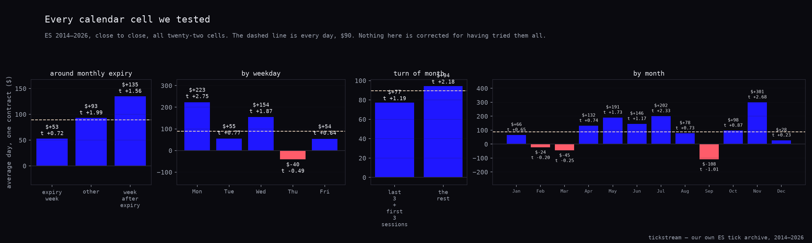
The chart below puts all four families side by side, each cell labelled with its average and its t. The dashed line on every panel is the all-days average of $89.65, and that is the line to read against rather than the zero axis. The fourth panel is every month of the year, November included, which is the other cell in this article that looks tradeable.
Pricing the search
Twenty-two cells were tested. At p = 0.05 you expect roughly one false positive per twenty tests by construction. A search this size is expected to hand you about one significant-looking cell even if the calendar carries no information at all. And you will find it, because you will look at all twenty-two and write about the one that won.
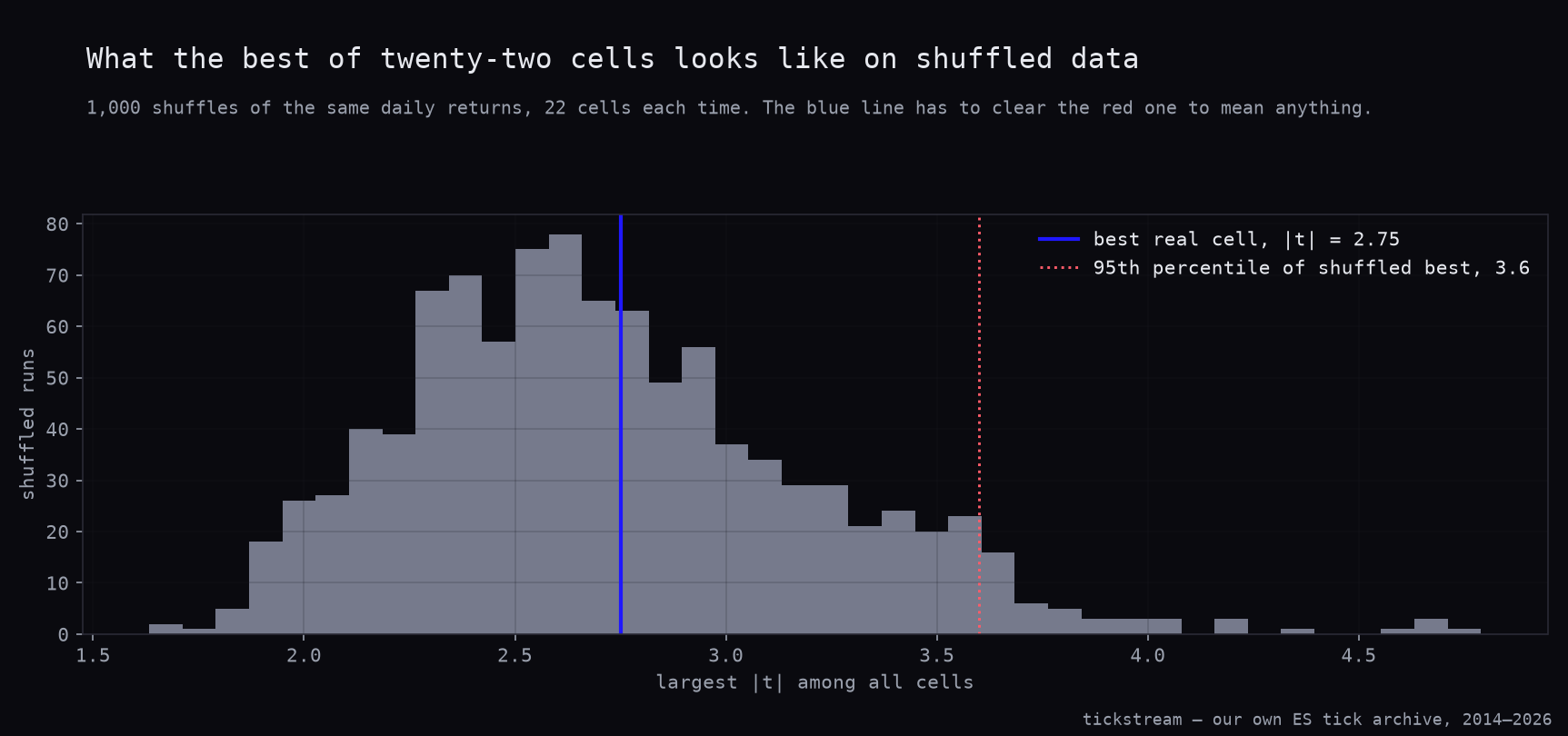
So we priced the search directly. We took the same 3,223 daily returns, shuffled them 1,000 times, and each time carved them into segments matching the sizes of our 22 real cells. Then we recorded the largest |t| in each shuffled run. That distribution is what “the best of 22 cells” looks like when the calendar means nothing.
| Pricing the whole search | |
|---|---|
| Cells tested | 22 |
| Best real cell, absolute t | 2.75 (Monday) |
| Best shuffled cell, mean absolute t | 2.72 |
| Best shuffled cell, 95th percentile | 3.60 |
| Shuffled runs beating our real best | 41.1% |
Our winner is 2.75. The average winner on shuffled data is 2.72. Four shuffled runs in ten produce a better best cell than the real calendar does, and clearing the 95th percentile would have required |t| of 3.60.
Monday’s p of 0.0061 is a perfectly good p-value for a single test specified in advance. As the winner of twenty-two it means nothing at all. Both statements are true about the same number, which is the part that makes multiplicity so easy to publish through.
This is now the standing rule for this series. When we test a family of cells, we report the best real cell against the best cell of the same family on shuffled data. The interesting number is never the winner’s p-value. It is the distribution of winners.
The regime model is the same lesson in different clothes
Split the same sessions by 20-day realised volatility against its own 250-day median, and the result looks like the cleanest finding on this page.
| Volatility regime | Sessions | Average | Up | t | p |
|---|---|---|---|---|---|
| Low vol | 1,638 | $120.74 | 54.3% | 3.76 | 0.0002 |
| High vol | 1,566 | $61.07 | 54.3% | 0.92 | 0.3555 |
p = 0.0002 on 1,638 sessions. Trade the quiet tape, sit out the loud one. The obvious next step is to build the filter — which is exactly what makes it worth building honestly.
So we chose the better regime on a rolling 500-day window and applied that choice forward, never using a day to decide about itself.
| Sessions | Average | Up | t | p | |
|---|---|---|---|---|---|
| Regime filter, walk-forward | 1,328 | $96.81 | 55.0% | 1.92 | 0.0551 |
| Hold everything, same span | 2,704 | $106.23 | 54.8% | 2.51 | 0.0121 |
The filter trades on half as many days, earns less on each of them, and loses the significance the in-sample split appeared to have. Doing nothing beat it on both figures that matter.
We published the same shape as a hidden Markov regime model on NQ, where the in-sample version looked strong and the walk-forward version fell below buy and hold. Two different regime definitions, two different instruments, one result. A regime model measured in hindsight beats holding; the same model measured forward does not. The gap between those two numbers is not a detail of the implementation. It is the entire subject.
What we changed
Nothing went into the book, and nothing was going to. What changed is the reporting standard.
- Every cell family now ships with its shuffled twin. Best real cell against best shuffled cell, in the article, next to the winner. If we cannot beat our own shuffled data we say the family is dead rather than quoting the survivor.
- We are retiring the post-expiry claim. Our internal, unpublished NQ read called it a modest survivor. On 448 post-expiry S&P sessions it pays $134.93 at t = 1.56, which is not enough to keep saying it. The extra five and a half years of ES is the reason we can say that at all, and this series exists to catch exactly this kind of thing.
- Regime filters are judged against the same span of buy and hold, walk-forward, or not at all. $96.81 versus $106.23 is the number that decides, not $120.74 versus $61.07.
A calendar effect we would actually trade has to do three things: name the forced flow that causes it, be specified before it is tested, and beat the best cell of its own shuffled family. None of the twenty-two here does the third, and only expiry seriously attempts the first.
The neighbouring test in this series is the ES gap study against a mirror control, with the original NQ gap-fill version for the second verdict.
The archive this ran on is for sale: ES ticks back to 2014 with the real aggressor side on every print, in the historical data packages.
Methodology: ES daily bars in New York time, built from our own tick archive, 3 January 2014 to 10 September 2026, 3,223 sessions. Each session’s P&L is the prior close to the open plus the open to the close, one contract, no stop and no filter. Cells are holds rather than trades, so no cost is charged within a cell; the series convention for a round trip is $4.50 commission plus two ticks, $29.50 on ES. Expiry week is the five sessions ending on the third Friday, the week after expiry the three sessions that follow it; turn of month is calendar days 26+ and 1–3. t-statistics are one-sample against zero on each cell’s daily series. The multiplicity test permutes the same 3,223 daily returns 1,000 times and records the largest |t| among 22 cells of matched sizes on each shuffle. Volatility regime is 20-day realised standard deviation against its own 250-day median; the walk-forward version picks the higher-mean regime from the trailing 500 sessions and applies it to the next session only.
Frequently asked questions
Is the Monday effect real on S&P futures?
Monday pays $223.19 a session over 642 Mondays, 58.6% of them up, at t = 2.75 and p = 0.0061. As a single planned test that is significant. As the best of the 22 calendar cells we measured it is not: the best cell on shuffled data averages |t| = 2.72, and 41.1% of shuffled runs produce a larger best cell than our real Monday.
Does the turn-of-month effect show up in the ES archive?
It shows up backwards. The last three and first three sessions of each month pay $77.20 a session over 886 sessions, while the other 2,337 sessions pay $94.37. Neither cell separates from the all-days baseline, and the turn-of-month bucket has the lower t of the two at 1.19.
Do post-expiry weeks still pay on the S&P?
Weakly. The week after monthly expiry pays $134.93 a session against $52.95 in expiry week and $93.13 in ordinary weeks, but at t = 1.56 and p = 0.1184 it does not clear significance. An internal NQ run of ours called post-expiry a modest survivor. We never published that run, so on this one the ES numbers stand alone, and at t = 1.56 they do not support the claim.
Which month is strongest on ES futures?
November, at $300.59 a session over 255 sessions with 61.6% of them up, t = 2.68. July is second at $201.92 and t = 2.33. Both sit inside the same 22-cell search that shuffled data beats 41.1% of the time, so neither is evidence of a November trade.
Does filtering for a low-volatility regime improve returns?
In hindsight, clearly. Low-volatility days pay $120.74 at t = 3.76 against $61.07 at t = 0.92 for high-volatility days. Chosen walk-forward on a rolling 500-day window, the same rule pays $96.81 a day at t = 1.92 while simply holding over that span pays $106.23 at t = 2.51 — less money per day, fewer days, and no significance.